I have been growing more interested in model calibration in recent times. For example, if a model says there is an 80% chance that a message is spam, I want to know what that number buys me. Could I use such model output to decide when software should act, when it should ask a person, and when it should leave the message alone?
TypeSafe's Jev was released only about two weeks ago and had a remarkably fast rise: Vercel called it the fastest-adopted model in AI Gateway history. Jev is built to give software typed decisions together with probabilities, rather than generate free-form text. Just two weeks later, OpenAI announced its Decisions API in limited preview, which I unfortunately don't have access to yet 😢. Then came Cloudflare's Clef on Oct 1st, an open-source decision model with a very similar question-and-answer interface.
That made for an irresistible little experiment: give Jev and Clef the same labeled text, ask them the same question, and see what their probabilities actually mean in practice.
First, what does “model calibration” mean?
Imagine sorting 100 messages into a pile because a model assigned each roughly 80% probability of spam. If about 80 of those messages really are spam, that pile is well calibrated. If only 40 are, the model is overestimating the chance of spam. If 95 are, it is underestimating it.
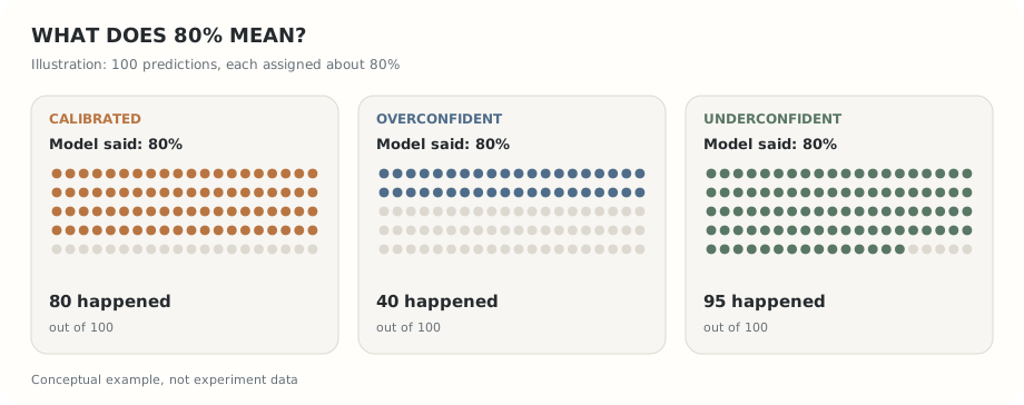
A probability expresses uncertainty about an individual outcome. Calibration asks whether, across many cases assigned similar probabilities, those probabilities line up with observed frequencies.
Accuracy asks whether the model picked the right side of a threshold. Calibration asks whether the numbers attached to its picks match what happens. A model can classify nearly everything correctly and still give probabilities that are too timid or too bold. That matters when different actions carry different costs: perhaps a 95% spam estimate is enough to hide a message, but a 60% estimate should send it to review.
What does Jev claim?
A central part of TypeSafe's pitch is that Jev returns calibrated probabilities. They use “calibrated” in the familiar statistical sense. Its AI primer says that outcomes assigned probability 0.8 should occur about 80% of the time across many predictions. The launch post calls the outputs “epistemically honest probabilities” for the narrow, fast judgments it calls System One tasks. I believe that a short sentiment or spam judgment is a reasonable test of that idea.
TypeSafe's workflow evaluations compare Jev with reference probabilities from other powerful models. That is useful for evaluating agreement on complex workflows, but it does not directly establish that Jev's 0.8 predictions occur 80% of the time against observed labels.
TypeSafe also exposes a separate confidence statistic for Choice and Score questions. It is derived from the shape of the returned probability distribution and should not be read as “the probability that the answer is correct.” My experiment uses Noul yes/no questions, which have no separate confidence field, so the quantity of interest is simply the model’s returned probability of “yes”: positive sentiment or spam.
Cloudflare makes a somewhat softer calibration claim for Clef: it says its post-training paired a Brier loss with cross-entropy to refine probability calibration and used RLCD as a secondary optimization target.
The experiment
I used two classic datasets from the UCI Machine Learning Repository: sentences labeled positive or negative, drawn from Amazon, IMDb, and Yelp reviews, and SMS messages labeled spam or legitimate. The sentiment dataset was deliberately assembled to contain clear positive or negative examples, so I expect it to be an easier test. The SMS dataset has a more realistic class imbalance.
After deduplication, I drew fixed-seed samples of 500 examples per task. Phone-like and email-like strings in the SMS text were replaced before sending messages to either API. Jev and Clef received the same text and the same yes/no question. For sentiment, it was: “Does this text express positive rather than negative sentiment?” For SMS: “Is this text message spam rather than a legitimate personal message?” I recorded each model's probability of “yes” and compared it with the supplied label.
I used 0.5 as the classification threshold. I treated ECCE-R, the range of a cumulative curve of observed outcomes minus predicted probabilities, as the main calibration diagnostic. Equal probability scores were grouped before evaluating that curve. I also looked at accuracy and the Brier score, the average squared error of the probabilities. Lower is better for ECCE-R and Brier. Brier mixes calibration with the ability to distinguish classes; ECCE-R focuses on calibration without choosing probability bins. I also checked ten-bin reliability tables, including each bin's sample size.
To see how stable the differences were on these rows, I resampled the same matched rows 2,000 times and recalculated each Jev-minus-Clef gap. Separately, I simulated 1,000 sets of outcomes as though each model's reported probabilities were perfectly calibrated. That second check asks whether the observed ECCE-R is unusually large relative to the sampling variation we would expect if those probabilities were correct; it does not directly compare the two models. I return to the assumptions behind both checks below.
The code and prompts are on GitHub if you want to download the public datasets and run the experiment with your own API access.
The first 100 were almost too easy
Both models classified all 100 items in the initial sentiment pilot correctly. That sounds impressive, but it provides little room to study uncertainty. When nearly every answer is obvious, a comparison of calibration can become a comparison of which model is willing to say 0.99 instead of 0.95.
Sentiment
500 sentencesClef leads on this unusually easy sample.
Redacted SMS
500 messagesAlways predicting “legitimate” would score 86.8% accuracy.
Five hundred sentiment sentences
On the larger matched sentiment sample, Jev classified 98.6% correctly and Clef 99.2%. For the positive class, precision was 98.8% versus 99.2%, and recall was 98.5% versus 99.2%. Their Brier scores were 0.0158 and 0.0077 respectively. Jev's ECCE-R was 0.0351 and Clef's 0.0122. The resampled differences appear together below.
The interesting detail is the direction. Jev was often underconfident about the positive label on this sample: its probabilities tended to be lower than the observed positive rate among comparable predictions. That is a calibration gap, even though its classification accuracy was excellent. Clef's probabilities were closer to the observed frequencies here.
The sentiment set's handpicked, clearly positive or negative sentences make this an unusually easy classification task. Both models exceeded 98% accuracy, so let's look at a slightly harder task.
A second task changes the picture
Spam is a better stress test because most messages are legitimate, and a false alarm may be costly. In the 500 redacted SMS messages, 13.2% carried the spam label. Yet the average predicted spam probability was 28.9% for Jev and 26.4% for Clef. Both overpredicted spam overall on this sample.
Jev classified 93.6% of messages correctly, compared with Clef's 85.6%, and had the better Brier score: 0.0634 versus 0.0991. ECCE-R went the other way: 0.1589 for Jev versus 0.1329 for Clef. Both sets of spam probabilities look poorly calibrated on this sample, but the models differ in how their classification and calibration errors trade off.
The class imbalance also makes accuracy easy to misread: predicting “legitimate” for every message would already get 86.8% right. At a 0.5 threshold, Jev caught 63 of 66 spam messages and Clef caught 62, but with quite different numbers of false positives. That threshold is not meant to be optimal, and optimizing it is not the point of this experiment. The main question here is calibration: whether a reported probability of, say, 70% behaves like 70% in practice. Thresholded precision, recall, and accuracy are included mainly as context for how the scores translate into one particular operating point.
One slice makes Jev's gap tangible. Among 134 messages it assigned spam probabilities between 0.1 and 0.2, the average prediction was about 0.133; only one message was labeled spam. Some examples labeled legitimate nevertheless read like promotions or chain messages, and replacing numbers and addresses may have removed context. That deserves a closer label review. It does not, on its own, explain the entire gap.
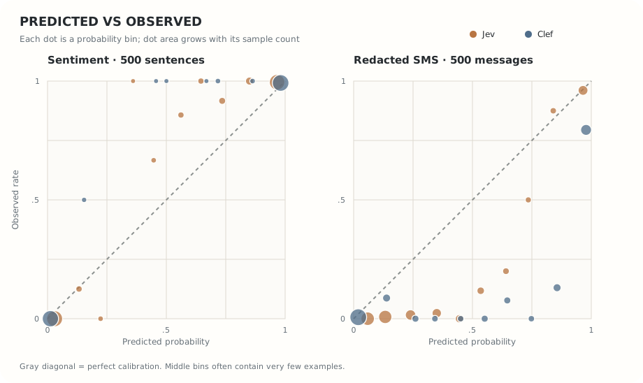
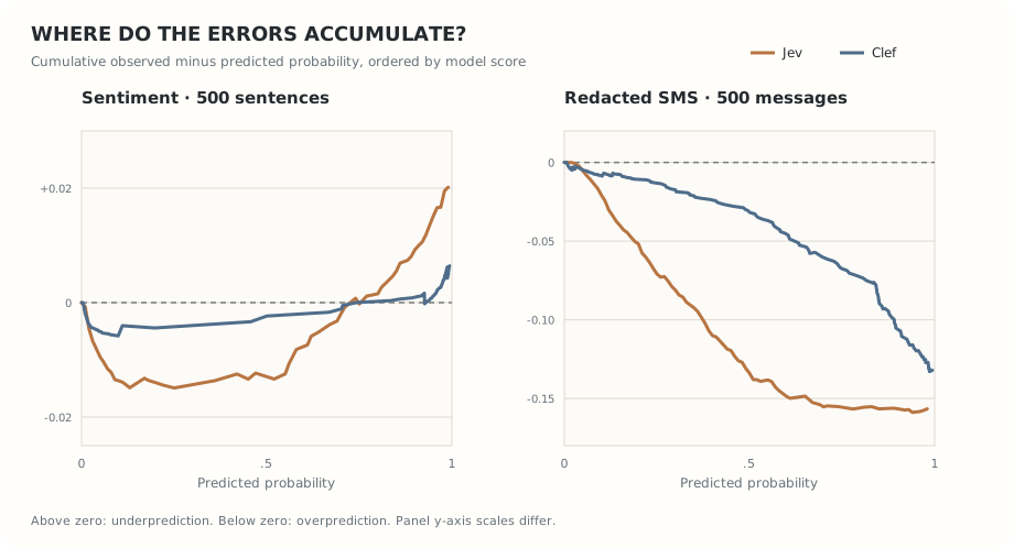
The ordering from sentiment does not carry over neatly. Better accuracy, better overall probability error, and better calibration can point in different directions. So can two tasks: “calibrated” is not a universal property that automatically transfers from one dataset to another.
How uncertain are the differences?
The table shows Jev minus Clef for the two measures most relevant to the probability question. Positive values favor Clef because lower error is better; negative values favor Jev. Each range covers the central 95% of 2,000 paired bootstrap resamples of the 500 matched rows.
| Task | Measure | Observed gap | Central 95% resampling range |
|---|---|---|---|
| Sentiment | ECCE-R | +0.0228 | +0.0165 to +0.0300 |
| Sentiment | Brier | +0.00815 | +0.00502 to +0.01170 |
| Redacted SMS | ECCE-R | +0.0260 | +0.0098 to +0.0421 |
| Redacted SMS | Brier | −0.03570 | −0.05063 to −0.02161 |
Treat these bootstrap ranges as a sense of stability rather than formal guarantees, since they do not capture uncertainty from choices like the input prompt, label noise introduced by redaction, or whether these widely used benchmark examples may have appeared in model pretraining.
Lastly, the calibrated-probability simulation serves as a model check. If each model's reported probabilities were perfectly calibrated, none of 1,000 simulations produced an ECCE-R as large as Jev's sentiment result or either model's SMS result; about 15% matched or exceeded Clef's sentiment result. Note that these checks are exploratory rather than confirmatory.
How much can this tell us?
These are small samples from old, public benchmarks for a little curiosity I wanted to satisfy. The sentiment set intentionally favors obvious cases, and either dataset may overlap material the models saw during pre-training. The supplied labels can also be imperfect, and redaction changes some SMS messages. Hence, these insights are not indicative of how these models would act in real production workflows. It also does not establish how either model behaves after a shift in language, prevalence, or user population.
Even good overall calibration can conceal trouble inside a subgroup. A model could look fine in aggregate while being overconfident on one kind of message and underconfident on another. See also MCGrad's work on multicalibration: checking and improving calibration across many slices of the data. Perhaps for a next blogpost.
What I take away
The appeal of decision models is real: fast, inexpensive answers to narrowly defined questions could be useful wherever the same judgment has to be made at scale. I like the idea of models that return usable probabilities instead of just scores. Jev and Clef make that idea very easy to test. But an API returning a number between zero and one does not automatically make that number dependable as a probability. Having labeled examples from the decision I actually care about, and checking those probabilities before setting an automated threshold, still seems useful for many use cases.
And if the raw scores are off, the story does not end there. Nothing stops us from fitting a calibrator on top of them, like MCGrad when we have useful features and enough data to examine subgroups.
The habit of asking what a probability means is worth keeping.
A quick note: The idea, questions, experimental design, and structure came from my own brain. AI was used as an assistant to rapidly run the experiments and help draft the post, something I’m actually excited to share. We can now go from “Wait, is that actually true?” to testing it surprisingly fast. What a time to be a curious scientist.